Accelerating Partitioning of Billion-scale Graphs with DGL v0.9.1

Graphs is ubiquitous to represent relational data, and many real-world applications such as recommendation and fraud detection involve learning from massive graphs. As such, GNNs has emerged as a powerful family of models to learn their representations. However, training GNNs on massive graphs is challenging, one of the issues is high resource demand to distribute graph data to a cluster. For example, partitioning a random graph of 1 billion nodes and 5 billion edges into 8 partitions requires a powerful AWS EC2 x1e.32xlarge instance (128 vCPU, 3.9TB RAM) running for 10 hours to finish the job.

In the latest DGL v0.9.1, we released a new pipeline for preprocess, partition and dispatch graph of billions of nodes or edges for distributed GNN training. At its core is a new data format called Chunked Graph Data Format (CGDF) which stores graph data by chunks. The new pipeline processes data chunks in parallel which not only reduces the memory requirement of each machine but also significantly accelerates the entire procedure. For the same random graph with 1B nodes/5B edges, using a cluster of 8 AWS EC2 x1e.4xlarge (16 vCPU, 488GB RAM each), the new pipeline can reduce the running time to 2.7 hours and cut down the money cost by 3.7x.

In this blog, we will illustrate step-by-step how to partition and distribute a graph of billions of nodes and edges using this new feature.

Distributed GNN Training 101

A graph dataset typically consists of graph structure and the features associated with nodes/edges. If the graph is heterogeneous (i.e., having multiple types of nodes or edges), different types of nodes/edges may have different sets of features. Training a GNN model on a multi-machine cluster first requires users to partition their input graph, which involves two steps:

1. Run a graph partition algorithm (e.g., random, METIS) to assign each node to one partition.
2. Shuffle and dispatch the graph structure and node/edge features to the target machine that owns the partition.

Once the graph is partitioned and provisioned, users can then launch the distributed training program using DGL’s launch tool, which will:

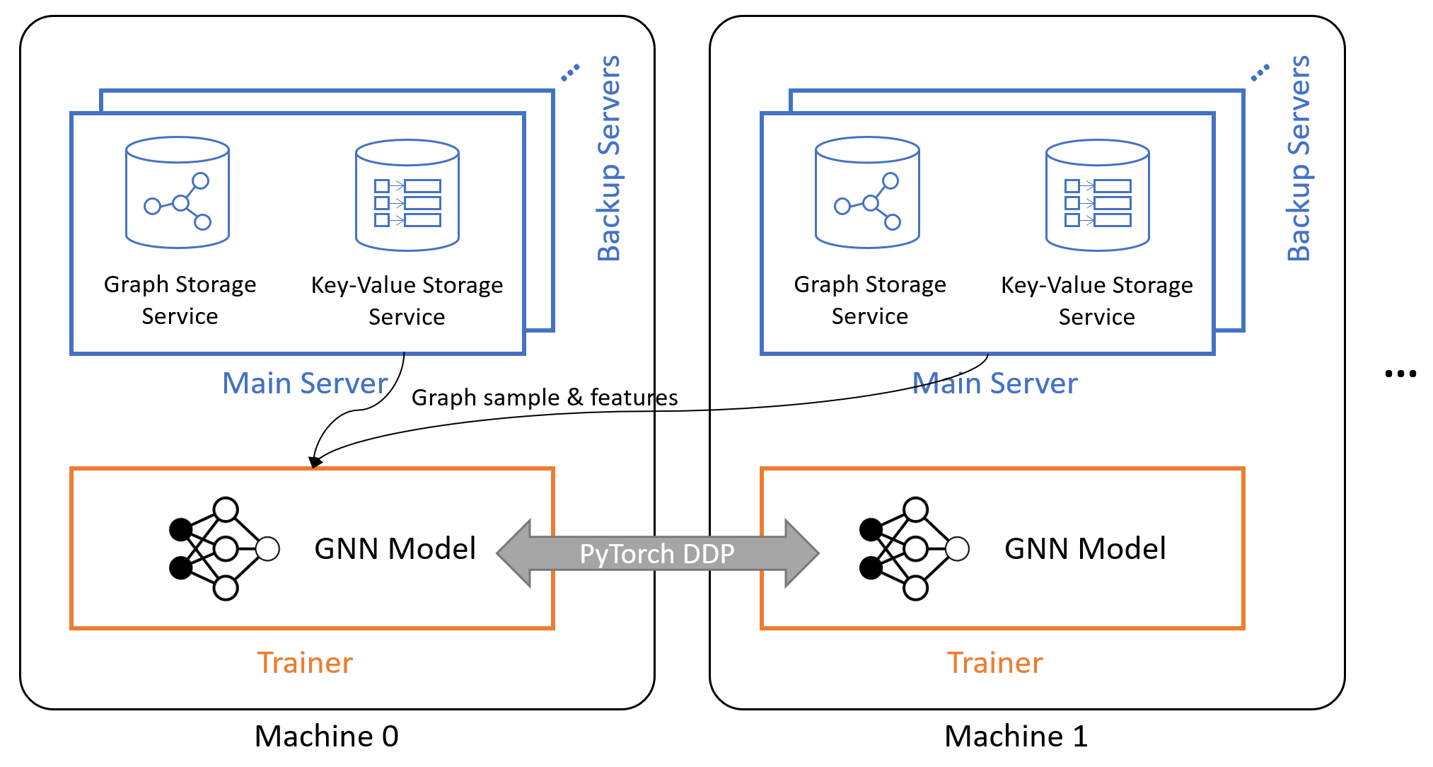
1. Launch one main graph server per machine that loads the local graph partition into RAM. Graph servers provide remove process calls (RPCs) to conduct computation like graph sampling. Optionally, users can launch more backup graph servers that share the in-memory data of the main graph server to increase service throughput.
2. Launch a key-value store (KVStore) server per machine that loads the local node/edge features into RAM. KVStore service provides RPCs to fetch/update node/edge features.
3. Launch one or more trainer processes per machine. Trainer processes are connected with each other via PyTorch’s DistributedDataParallel component. At each training iteration, they issue requests to local or remote graph servers and KVStore servers to get a mini-batch of samples, perform gradient descent and synchronize their gradients before the next iteration.

The figure below depicts the system architecture. For more information, check out the Distributed Training chapter of DGL User Guide.

Due to the complexity of graph data, graph partitioning is typically run on a single machine, which demands the machine to have large enough memory to fit the entire graph and features as well as the runtime usage from the partition algorithm. For example, a random graph of 1 billion nodes and 5 billions edges and 50 features per nodes needs 268GB when stored in DGL graph format. Using the existing dgl.distributed.partition_graph API to partition this graph requires a powerful AWS EC2 x1e.32xlarge instance (128 vCPU, 3.9TB RAM) and runs for 10 hours — a significant bottleneck for users to train GNNs at scale.

DGL v0.9.1 addressed the issue by a new distributed graph partitioning pipeline. Specifically,

• We designed a Chunked Graph Data Format (CGDF) for storing large graph data in chunks to avoid loading the entire graph into a single machine.
• We provided scripts to partition and dispatch chunked graph in parallel using multiple machines to reduce the memory requirement of each machine as well as to accelerate the procedure.

Chunked Graph Data Format

Chunked graph dataset is organized as a data folder with the following data files:

• A metadata.json file that stores the meta information of the graph, e.g., graph name, node/edge types, chunk sizes, chunk file paths, etc.
• A list of edge index chunk files that store the source and destination node IDs. They are typically in plain texts.
• A list of node data chunk files. They are typically array data stored in NumPy array binary.
• A list of edge data chunk files. They are also in NumPy array binary.

Here, we illustrate the folder structure and the data files of a random social graph (nodes being users, edges being follow relation) where nodes have two data: “feat” and “label”. Check out the doc page for the full specification of the format and tips for how to convert your data to chunks.

//data/random_graph_chunked/
  |-- metadata.json            # metadata JSON
  |-- edge_index/              # edge index chunks
    |-- user:follow:user0.txt  # user-follow-user edges chunk 0
    |-- user:follow:user1.txt  # user-follow-user edges chunk 1
    |-- user:follow:user2.txt  # user-follow-user edges chunk 2
    |-- ...
  |-- node_data/           # node data chunks
    |-- user/              # user nodes have two data: "feat" and "label"
      |-- feat0.npy        # feat chunk 0
      |-- feat1.npy        # feat chunk 1
      |-- feat2.npy        # feat chunk 2
      |-- ...
      |-- label0.npy       # label chunk 0
      |-- label1.npy       # label chunk 1
      |-- label2.npy       # label chunk 2
      |-- ...
  |-- edge_data/           # edge data chunks
    |-- user:follow:user/
       |-- ...

Running Distributed Partitioning & Dispatching

The first step is to get a cluster of machines to partition the graph. We recommend the total RAM size of the cluster to be 2-3x larger than the graph data size to accommodate the runtime memory needed. Next is to setup shared workspace and software environment.

1. Setup a shared folder that is accessible by each instance in the cluster (e.g., using NFS). Make sure all instances can ssh to each other. Here, we suppose the folder is mounted to /workspace.
2. Clone and download the scripts from DGL 0.9.x branch to /workspace:

   git clone https://github.com/dmlc/dgl.git -b 0.9.x /workspace/dgl
   

3. Copy/move the chunked graph data to /workspace/. Here, we suppose the data folder is at /workspace/random_graph_chunked/.
4. Create an /workspace/ip_config.txt file that contains the IP address of each instance.

   # example IP config file of a 4 machine cluster
   172.31.19.1
   172.31.23.205
   172.31.29.175
   172.31.16.98
   

We can then run a partition algorithm to assign each node to a partition. Here, we choose random partitioning algorithm.

python /workspace/dgl/tools/partition_algo/random_partition.py \
    --in_dir=/workspace/random_graph_chunked/
    --out_dir=/workspace/partition_assign/
    --num_partitions=4

The above script simply calculates which partition a node belongs to. We then pass both the chunked graph and the partition assignments to the dispatch_data.py script to physically split the graph data into multiple pieces and distribute them to the entire cluster.

python /workspace/dgl/tools/dispatch_data.py \
    --in-dir=/workspace/random_graph_chunked/
    --partitions-dir=/workspace/partition_assign/
    --out-dir=/workspace/random_graph_dist/
    --ip-config=/workspace/ip_config.txt

The end result will look like the following. We can then launch distributed training following the instructions here.

/workspace/random_graph_dist/
  |-- medatdata.json      # metadata JSON file
  |-- part0/              # partition 0
    |-- graph.dgl         # graph structure of partition 0 in DGL binary format
    |-- node_feat.dgl     # node feature of partition 0 in DGL binary format
    |-- edge_feat.dgl     # edge feature of partition 0 in DGL binary format
  |-- part1/              # partition 1
    |-- graph.dgl         # graph structure of partition 1 in DGL binary format
    |-- node_feat.dgl     # node feature of partition 1 in DGL binary format
    |-- edge_feat.dgl     # edge feature of partition 1 in DGL binary format
  |-- part2/
  ...

Note that the scripts utilize multiple machines to cooperatively partition and process the data. Therefore, the new pipeline is significantly faster. For the same random graph with 1B nodes/5B edges, the new pipeline can finish partitioning in 2.7 hours (3.7x faster) using an cluster of 8 AWS EC2 x1e.4xlarge (16 vCPU, 488GB RAM).

Further Readings

• User guide for the new distributed graph partitioning pipeline.
• Example for training a GraphSAGE model on a cluster of machines.
• Other enhancement in the latest v0.9.1 release.