v0.9 Release Highlights

Six years after the first Graph Convolutional Networks paper, researchers are actively investigating more advanced GNN architecture or training methodology. As the developer team of DGL, we closely watch those new research trends and release features to facilitate them. Here, we highlighted some of the new functionalities of the recent v0.9 release.

Combining Graph Analytics with GNNs using cuGraph+DGL

Graph neural networks (GNNs) are capable of combining the feature and structural information of graph data. Its power can be further extended when synergistically combined with techniques of graph analytics, such as feature augmentation.

Graph analytics has been widely used for characterising graph structures, e.g., identifying important nodes, leading to interesting feature augmentation methods. To exploit the synergy, we would want a fast and scalable graph analytics engine. NVidia’s RAPIDS cuGraph library provides a collection of GPU accelerated algorithms for graph analytics, such as centrality computation and community detection. According to this documentation, “the latest NVIDIA GPUs (RAPIDS supports Pascal and later GPU architectures) make graph analytics 1000x faster on average over NetworkX”.

With collaboration with NVidia’s engineers, DGL v0.9 now allows conversion between a DGLGraph object and a cuGraph graph object with two APIs to_cugraph and from_cugraph, making it possible for DGL users to access efficient graph analytics implementations in cuGraph.

Installation

To install cuGraph with PyTorch and DGL, we recommend following the practice below. Mamba is a multi-threaded version of conda.

conda install mamba -n base -c conda-forge

mamba create -n dgl_and_cugraph -c dglteam -c rapidsai-nightly -c nvidia -c pytorch -c conda-forge \
    cugraph pytorch torchvision torchaudio cudatoolkit=11.3 dgl-cuda11.3 tqdm

conda activate dgl_and_cugraph

Feature Initialization via cuGraph

We showcase an example of node feature initialization using the graph analytics algorithms provided by cuGraph. Here, we consider two options:

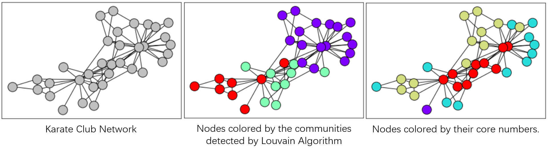
• Louvain algorithm that detects the community membership of each node based on modularity optimization.
• Core number algorithm that calculates the maximal k-core subgraph each node belongs to. A k-core of a graph is a maximal subgraph that contains nodes of degree k or more.

The two algorithms capture different structural characteristics of a node. Louvain groups nodes with close spatial distance with each other, while nodes with the same core numbers are more structurally similar with each other. The figures below illustrate the node coloring produced by Louvain communities and core numbers on Zachary’s Karate Club Network.

cuGraph offers efficient GPU implementations of these two algorithms. To call them, we convert a dgl.DGLGraph to a cugraph.Graph using the to_cugraph API.

import cugraph
import torch

def louvain(dgl_g):
    cugraph_g = dgl_g.to_cugraph().to_undirected()
    df, _ = cugraph.louvain(cugraph_g, resolution=3)
    # revert the node ID renumbering by cugraph
    df = cugraph_g.unrenumber(df, 'vertex').sort_values('vertex')
    return torch.utils.dlpack.from_dlpack(df['partition'].to_dlpack()).long()

def core_number(dgl_g):
    cugraph_g = dgl_g.to_cugraph().to_undirected()
    df = cugraph.core_number(cugraph_g)
    # revert the node ID renumbering by cugraph
    df = cugraph_g.unrenumber(df, 'vertex').sort_values('vertex')
    return torch.utils.dlpack.from_dlpack(df['core_number'].to_dlpack()).long()

Training GNN via DGL

We then use the above functions to prepare node features for the ogbn-arxiv dataset. Note that since both algorithms calculate structural categories, we convert them to one-hot encoding and concatenate them as the initial node features.

import dgl.transforms as T
import torch.nn as nn
import torch.nn.functional as F

from dgl.nn import SAGEConv
from ogb.nodeproppred import DglNodePropPredDataset, Evaluator

device = torch.device('cuda')
dataset = DglNodePropPredDataset(name='ogbn-arxiv')
g, label = dataset[0]
transform = T.Compose([
    T.AddReverse(),
    T.AddSelfLoop(),
    T.ToSimple()
])
g = transform(g).int().to(device)
feat1 = louvain(g)
feat2 = core_number(g)
# convert to one-hot
feat1 = F.one_hot(feat1, feat1.max() + 1)
feat2 = F.one_hot(feat2, feat2.max() + 1)
# concat feat1 and feat2
x = torch.cat([feat1, feat2], dim=1).float()

We then train a simple three layer GraphSAGE model (see complete training code here). With the help of node features initialized by graph analytics algorithms, we are able to achieve an accuracy of about 0.6 on the test set using pure structural information, which even outperforms an MLP model using the original input node features. With the new DGL release, we are looking forward to seeing more innovation on GNNs combined with graph analytics.

FP16 & Mixed Precision Support

DGL v0.9 is now fully compatible with the PyTorch Automatic Mixed Precision (AMP) package for mixed precision training, thus saving both training time and GPU memory consumption.

By wrapping the forward pass with torch.cuda.amp.autocast(), PyTorch automatically selects the appropriate data type for each op and tensor. Half precision tensors are memory efficient, most operators on half precision tensors are faster as they leverage GPU tensorcores.

import torch.nn.functional as F
from torch.cuda.amp import autocast

def forward(g, feat, label, mask, model):
    with autocast(enabled=True):
        logit = model(g, feat)
        loss = F.cross_entropy(logit[mask], label[mask])
        return loss

Small gradients in float16 format have underflow problems (flush to zero). PyTorch AMP provides a GradScaler module to address this issue. It multiplies the loss by a factor and invokes backward pass on the scaled loss to prevent the underflow problem. It then unscales the computed gradients before the optimizer updates the parameters. The scale factor is determined automatically.

from torch.cuda.amp import GradScaler

scaler = GradScaler()

def backward(scaler, loss, optimizer):
    scaler.scale(loss).backward()
    scaler.step(optimizer)
    scaler.update()

Putting everything together, we have the example below.

import torch
import torch.nn as nn
from dgl.data import RedditDataset
from dgl.nn import GATConv
from dgl.transforms import AddSelfLoop

class GAT(nn.Module):
    def __init__(self, in_feats, num_classes, num_hidden=256, num_heads=2):
        super().__init__()
        self.conv1 = GATConv(in_feats, num_hidden, num_heads, activation=F.elu)
        self.conv2 = GATConv(num_hidden * num_heads, num_hidden, num_heads)

    def forward(self, g, h):
        h = self.conv1(g, h).flatten(1)
        h = self.conv2(g, h).mean(1)
        return h

device = torch.device('cuda')

transform = AddSelfLoop()
data = RedditDataset(transform)

g = data[0]
g = g.int().to(device)
train_mask = g.ndata['train_mask']
feat = g.ndata['feat']
label = g.ndata['label']
in_feats = feat.shape[1]

model = GAT(in_feats, data.num_classes).to(device)
model.train()
optimizer = torch.optim.Adam(model.parameters(), lr=1e-3, weight_decay=5e-4)

for epoch in range(100):
    optimizer.zero_grad()
    loss = forward(g, feat, label, train_mask, model)
    backward(scaler, loss, optimizer)

Training GNNs using low precision or mixed precision is still an active research topic. We hope the new v0.9 release will facilitate more research on this topic. Check out the documentation to know more.

DGL-Go Update: Model Inference and Graph Prediction

DGL-Go now supports training GNNs for graph property prediction tasks. It includes two popular GNN models – Graph Isomorphism Network (GIN) and Principal Neighborhood Aggregation (PNA). For example, to train a GIN model on the ogbg-molpcba dataset, first generate a YAML configuration file using command:

dgl configure graphpred --data ogbg-molpcba --model gin

which generates the following configuration file. Users can then manually adjust the configuration file.

version: 0.0.2
pipeline_name: graphpred
pipeline_mode: train
device: cpu                     # Torch device name, e.g., cpu or cuda or cuda:0
data:
    name: ogbg-molpcba
    split_ratio:                # Ratio to generate data split, for example set to [0.8, 0.1, 0.1] for 80% train/10% val/10% test. Leave blank to use builtin split in original dataset
model:
     name: gin
     embed_size: 300            # Embedding size
     num_layers: 5              # Number of layers
     dropout: 0.5               # Dropout rate
     virtual_node: false        # Whether to use virtual node
general_pipeline:
    num_runs: 1                 # Number of experiments to run
    train_batch_size: 32        # Graph batch size when training
    eval_batch_size: 32         # Graph batch size when evaluating
    num_workers: 4              # Number of workers for data loading
    optimizer:
        name: Adam
        lr: 0.001
        weight_decay: 0
    lr_scheduler:
        name: StepLR
        step_size: 100
        gamma: 1
    loss: BCEWithLogitsLoss
    metric: roc_auc_score
    num_epochs: 100             # Number of training epochs
    save_path: results          # Directory to save the experiment results

Alternatively, users can fetch model recipes of pre-defined hyperparameters for the original experiments.

dgl recipe get graphpred_pcba_gin.yaml

To launch training:

dgl train --cfg graphpred_ogbg-molpcba_gin.yaml

Another addition is a new command to conduct inference of a trained model on some other dataset. For example, the following shows how to apply the GIN model trained on ogbg-molpcba to ogbg-molhiv:

# Generate an inference configuration file from a saved experiment checkpoint
dgl configure-apply graphpred --data ogbg-molhiv --cpt results/run_0.pth

# Apply the trained model for inference
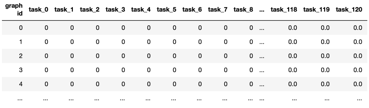
dgl apply --cfg apply_graphpred_ogbg-molhiv_pna.yaml

It will save the model prediction in a CSV file like below

Further Reading

Full release note: https://github.com/dmlc/dgl/releases/tag/0.9.0