v0.8 Release Highlights

We are excited to announce the release of DGL v0.8, which brings many new features as well as improvement on system performance. The highlights are:

• A major update of the mini-batch sampling pipeline, better customizability, more optimizations; 3.9x and 1.5x faster for supervised and unsupervised GraphSAGE on OGBN-Products, with only one line of code change.
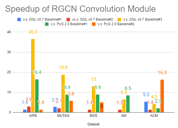
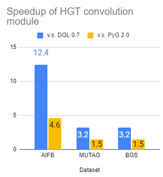
• Significant acceleration and code simplification of popular heterogeneous graph NN modules (Up to 36x for RGCN convolution and 12x for HGT convolution). 11 new off-the-shelf NN modules for building models for link prediction, heterogeneous graph learning and GNN explanation.
• GNNLens: a DGL empowered tool to visualize and understand graph data using GNN explanation models.
• New functions to create, transform and augment graph datasets, making it easier to conduct research on graph contrastive learning or repurposing a graph for different tasks.
• DGL-Go: a new GNN model training command line tool that utilizes a simple interface so that users can quickly apply GNNs to their problems and orchestrate experiments with state-of-the-art GNN models.

Mini-batch Sampling Pipeline Update

In training Neural Networks, minibatch sampling has been used to both improve model performance and enable scaling to large datasets. Mini-batch training in the context of GNNs on graphs introduces new complexities, which can be broken down into four main steps:

1. Extract a subgraph from the original graph.
2. Perform transformations on the subgraph.
3. Fetch the node/edge features of the subgraph.
4. Pass the subgraph and its features as the input to your GNN model and update parameters.

Among them, steps 1-3 are unique to GNNs and are quite costly. In v0.7, we have released the feature to speedup step 2 by transforming subgraphs on GPU, but the other two may continue to be the bottleneck. In this release, we further optimized the entire pipeline to reach an even better performance. We then briefly describe our technical solutions behind that.

To speed up subgraph extraction, we utilized CUDA Unified Virtual Addressing(UVA).

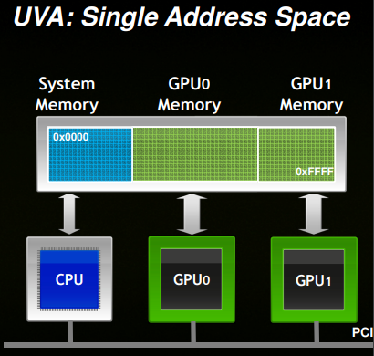
(Image courtesy: https://developer.download.nvidia.cn/CUDA/training/cuda_webinars_GPUDirect_uva.pdf)

CUDA UVA allows users to create in-memory data beyond the size of GPU RAM capacity while still harnessing GPU kernels for fast computation. Storing the entire graph structure and its features in UVA enables efficient subgraph extraction using GPU kernels, which is effective for training large-scale GNNs [1][2]. In this release, users can turn on the UVA mode by setting the use_uva flag in DataLoader, as shown in the example below:

g = ...                  # some DGLGraph data
train_nids = ...         # training node IDs
sampler = dgl.dataloading.MultiLayerNeighborSampler(
    fanout=[10, 15])
dataloader = dgl.dataloading.DataLoader(
    g, train_nids, sampler,
    device='cuda:0',     # perform sampling on GPU 0
    batch_size=1024,
    shuffle=True,
    use_uva=True         # turn on UVA optimization
)

To speed up feature fetching (step 3), DGL 0.8 supports pre-fetching node/edge features so that the model computation can happen in parallel with data movement. Users can specify the features as well as the labels to prefetch in the sampler object.

g = ...           # some DGLGraph data
train_nids = ...  # training node IDs
sampler = dgl.dataloading.MultiLayerNeighborSampler(
    fanout=[10, 15],
    prefetch_node_feats=['feat'],   # prefetch node feature 'feat'
    prefetch_labels=['label'],      # prefetch node label 'label'
)
dataloader = dgl.dataloading.DataLoader(
    g, train_nids, sampler,
    device='cuda:0',     # perform sampling on GPU 0
    batch_size=1024,
    shuffle=True,
    use_uva=True         # turn on UVA optimization
)

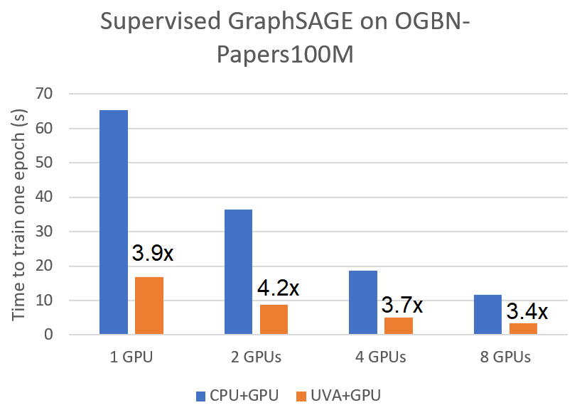
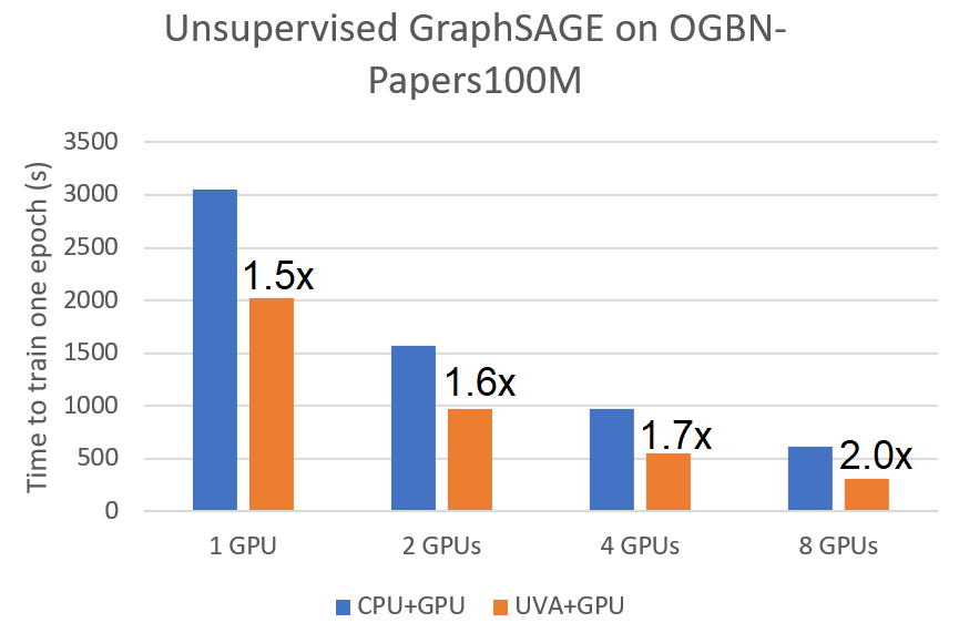
These optimizations bring significant speedup for both supervised and unsupervised mini-batch training. We compared it against the original pipeline of sampling on CPU but training on GPU for training a two-layer GraphSAGE model on the ogbn-papers100M graph using A100 GPUs. We observed a speedup of 3.9x and 1.5x for supervised and unsupervised GraphSAGE on a single GPU respectively. The speedup applies to multi-GPU training as well.

Speedup of Supervised GraphSAGE	Speedup of Unsupervised GraphSAGE

Defining a new sampler in DGL v0.8 is also easier, with only one simple interface sample to follow. Optionally, users can specify how to prefetch features for each sample. For example, the cluster sampler used by Cluster-GCN can be implemented in just a few lines of code.

class ClusterGCNSampler:
    def __init__(self, g, k, prefetch_ndata=None):
        part_ids = dgl.metis_partition_assignment(g, k)
        # convert partition assignment to bins of nodes
        part_sizes = torch.histogram(part_ids.float(), k)[0].int()
        self.node_bins = torch.split(torch.argsort(part_ids), part_sizes)
        # save the node feature names to be prefetched
        self.prefetch_ndata = prefetch_ndata

    def sample(self, g, part_ids):
        """Sample a subgraph given a list of partition IDs."""
        node_ids = torch.cat([self.node_bins[pid] for pid in part_ids])
        sg = g.subgraph(node_ids)  # get an induced subgraph
        # tell which feature to pre-fetch
        dgl.set_node_lazy_feature(sg, self.prefetch_ndata)
        return sg

New samplers in v0.8:

• dgl.dataloading.ClusterGCNSampler: The sampler from Cluster-GCN: An Efficient Algorithm for Training Deep and Large Graph Convolutional Networks.
• dgl.dataloading.ShaDowKHopSampler: The sampler from Deep Graph Neural Networks with Shallow Subgraph Samplers.

This remarkable improvement would not happen without the help from the community. We want to thank Xin Yao (@yaox12) and Dominique LaSalle (@nv-dlasalle) from NVIDIA and David Min (@davidmin7) from UIUC for their contributions.

Further reading:

• User guide chapter for customizing graph samplers.
• User guide chapter for writing graph samplers with feature prefetching.
• Example implementation of ClusterGCN.

NN Module Update

Heterogeneous GNNs are known to be both difficult to implement as well as difficult to optimize. In this release, we have significantly improved the speed of dgl.nn.RelGraphConv and dgl.nn.HGTConv – two state-of-the-art NN modules for training on heterogeneous graphs, by sometimes an order of magnitude compared with various baselines[3]:

Speedup of RGCN convolution	Speedup of HGT convolution

More importantly, writing an efficient heterogeneous graph convolution is substantially easier. Here is a minimal implementation of RGCN convolution in 0.8 using the new nn.TypedLinear module:

class RGCNConv(nn.Module):
    def __init__(self, in_size, out_size, num_etypes):
        # TypedLinear is a new module in 0.8!
        self.linear_r = dgl.nn.TypedLinear(in_size, out_size, num_etypes)

    def forward(self, g, x, etype):
        g.ndata['x'] = x
        g.edata['etype'] = etype
        g.update_all(self.message, dgl.function.sum('m', 'h'))
        return g.ndata['h']

    def message(self, edges):
        return self.linear_r(edges.src['h'], edges.data['etype'])

This release also brings 11 new NN modules covering the most requested ones from the community. They include but are not limited to:

• Commonly used edge score modules (e.g., TransE, TransR, etc.) for link prediction.
• Linear projection module and embedding module for heterogeneous graphs (nn.HeteroLinear and nn.HeteroEmbedding).
• The GNNExplainer module.

Understand Graph via Visualisation and GNN-based Explanation

Understanding graph data using GNN-based explanation model has become an important research topic. We partnered with the HKUST VisLab team to release GNNLens, an interactive visualization tool for graph neural networks.

To install GNNLens, pip install gnnlens.

It provides Python APIs for specifying the data to be visualized. For example, the following shows how to load DGL’s built-in Cora graph dataset and visualize it:

from dgl.data import CoraGraphDataset
dataset = CoraGraphDataset()
G = dataset[0]

from gnnlens import Writer

# Specify the path to create a new directory for dumping data files.
writer = Writer('tutorial_graph')
writer.add_graph(name='Cora', graph=cora_graph)
writer.add_graph(name='Citeseer', graph=citeseer_graph)
# Finish dumping
writer.close()

After running the script, you can then launch GNNLens with the following command:

gnnlens --logdir tutorial_graph

And you will see the webpage in your browser:

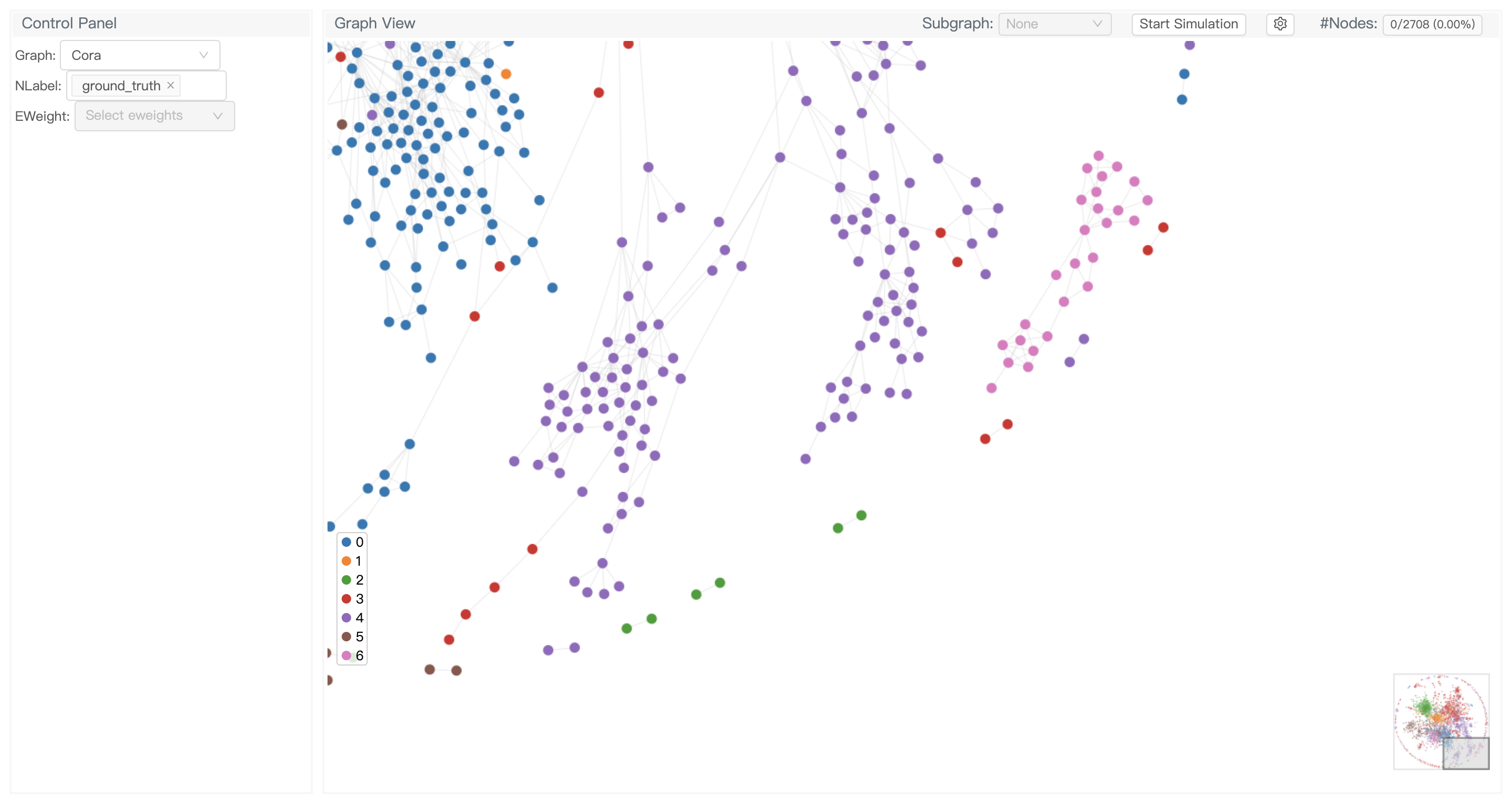
GNNLens is not only capable of visualizing raw graph data, but also designed for inspecting graph neural networks such as running explanation models to explain the prediction. Please check out the tutorials in the project README: https://github.com/dmlc/gnnlens2.

Composable Graph Data Transforms

Graph data augmentation has become an important component for graph contrastive learning or structural prediction in general. The new release makes it easier to compose and apply various graph augmentation and transformation algorithms to all DGL’s built-in dataset. The new dgl.transforms package follows the style of the PyTorch Dataset Transforms. Users can specify the transforms to use with the transform keyword argument of all DGL datasets:

import dgl
import dgl.transforms as T
t = T.Compose([
    T.AddSelfLoop(),
    T.GCNNorm(),
])
dataset = dgl.data.CoraGraphDataset(transform=t)
g = dataset[0]  # graph and features will be transformed automatically

DGL v0.8 provides 16 commonly used data transform APIs. See the API doc for more information.

Making graph datasets easily accessible for all kinds of research is important. A common scenario is to adapt a dataset for a different task than it was originally designed for (e.g., training a link prediction model on Cora which is originally for node classification). We therefore add two dataset adapters (dgl.data.AsNodePredDataset and dgl.data.AsLinkPredDataset) for this purpose. We also support generating new train/val/test split and save them for later use:

import dgl
dataset = dgl.data.CoraGraphDataset()
# make a Cora dataset suitable for link prediction
# add train/val/test split and negative samples
dataset = dgl.data.AsLinkPredDataset(dataset, split_ratio=[0.8, 0.1, 0.1], neg_ratio=3)

One more thing

As GNN is still a young and blooming domain, we received many “how to start” questions from our users:

• “I’ve heard about GNNs, how to start training a GNN model on my own datasets?”
• “I want to learn more about GNNs, how to start experimenting with SOTA baselines?”
• “I have some new research ideas, how to start building it upon existing GNN models?”

To make those first steps easier, we developed DGL-Go, a command line tool for users to quickly access the latest GNN research progress.

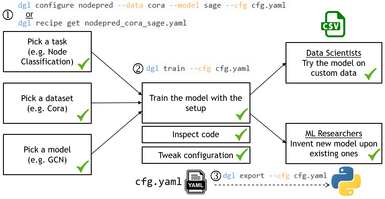
Using DGL-Go is as easy as three steps:

1. Use dgl configure to pick the task, dataset and model of your interests. It generates a configuration file for later use. You could also use dgl recipe get to retrieve a configuration file we provided.
2. Use dgl train to launch training according to the configuration and see the results.
3. Use dgl export to generate a self-contained, reproducible Python script for advanced customization, or try the model on custom data stored in CSV format.

Install DGL-Go simply by pip install dglgo and check out the project README for more details.

Further Reading

The full release note of DGL v0.8.

Reference

[1] PyTorch-Direct: Enabling GPU Centric Data Access for Very Large Graph Neural Network Training with Irregular Accesses

[2] TorchQuiver: https://github.com/quiver-team/torch-quiver

[3] We compared our new nn.RelGraphConv module with multiple existing baselines from DGL and PyG. For DGL v0.7, Baseline#1 uses the old nn.RelGraphConv module with low_mem=False; Baseline#2 uses the old nn.RelGraphConv with low_mem=True; Baseline#3 uses nn.HeteroGarphConv. For PyG, Baseline#1 uses nn.RGCNConv while Baseline#2 uses nn.FastRGCNConv. All the benchmarks are tested on one NVIDIA T4 GPU card.