Understand Graph Attention Network
From Graph Convolutional Network (GCN), we learned that combining local graph structure and node-level features yields good performance on node classification task. However, the way GCN aggregates is structure-dependent, which may hurt its generalizability.
One workaround is to simply average over all neighbor node features as in GraphSAGE. Graph Attention Network proposes an alternative way by weighting neighbor features with feature dependent and structure free normalization, in the style of attention.
The goal of this tutorial:
- Explain what is Graph Attention Network.
- Demonstrate how it can be implemented in DGL.
- Understand the attentions learnt.
- Introduce to inductive learning.
Introducing Attention to GCN
The key difference between GAT and GCN is how the information from the one-hop neighborhood is aggregated.
For GCN, a graph convolution operation produces the normalized sum of the node features of neighbors:
where is the set of its one-hop neighbors (to include in the set, simply add a self-loop to each node), is a normalization constant based on graph structure, is an activation function (GCN uses ), and is a shared weight matrix for node-wise feature transformation. Another model proposed in GraphSAGE employs the same update rule except that they set .
GAT introduces the attention mechanism as a substitute for the statically normalized convolution operation. Below are the equations to compute the node embedding of layer from the embeddings of layer :
Explanations:
- Equation (1) is a linear transformation of the lower layer embedding and is its learnable weight matrix.
- Equation (2) computes a pair-wise unnormalized attention score between two neighbors. Here, it first concatenates the embeddings of the two nodes, where denotes concatenation, then takes a dot product of it and a learnable weight vector , and applies a LeakyReLU in the end. This form of attention is usually called additive attention, contrast with the dot-product attention in the Transformer model.
- Equation (3) applies a softmax to normalize the attention scores on each node’s in-coming edges.
- Equation (4) is similar to GCN. The embeddings from neighbors are aggregated together, scaled by the attention scores.
There are other details from the paper, such as dropout and skip connections. For the purpose of simplicity, we omit them in this tutorial and leave the link to the full example at the end for interested readers.
In its essence, GAT is just a different aggregation function with attention over features of neighbors, instead of a simple mean aggregation.
GAT in DGL
Let’s first have an overall impression about how a GATLayer module is
implemented in DGL. Don’t worry, we will break down the four equations above
one-by-one.
import torch
import torch.nn as nn
import torch.nn.functional as F

class GATLayer(nn.Module):
    def __init__(self, g, in_dim, out_dim):
        super(GATLayer, self).__init__()
        self.g = g
        # equation (1)
        self.fc = nn.Linear(in_dim, out_dim, bias=False)
        # equation (2)
        self.attn_fc = nn.Linear(2 * out_dim, 1, bias=False)

    def edge_attention(self, edges):
        # edge UDF for equation (2)
        z2 = torch.cat([edges.src['z'], edges.dst['z']], dim=1)
        a = self.attn_fc(z2)
        return {'e' : F.leaky_relu(a)}

    def message_func(self, edges):
        # message UDF for equation (3) & (4)
        return {'z' : edges.src['z'], 'e' : edges.data['e']}

    def reduce_func(self, nodes):
        # reduce UDF for equation (3) & (4)
        # equation (3)
        alpha = F.softmax(nodes.mailbox['e'], dim=1)
        # equation (4)
        h = torch.sum(alpha * nodes.mailbox['z'], dim=1)
        return {'h' : h}

    def forward(self, h):
        # equation (1)
        z = self.fc(h)
        self.g.ndata['z'] = z
        # equation (2)
        self.g.apply_edges(self.edge_attention)
        # equation (3) & (4)
        self.g.update_all(self.message_func, self.reduce_func)
        return self.g.ndata.pop('h')
Equation (1)
The first one is simple. Linear transformation is very common and can be easily
implemented in Pytorch using torch.nn.Linear.
Equation (2)
The unnormalized attention score is calculated using the embeddings of
adjacent nodes and . This suggests that the attention scores can be
viewed as edge data which can be calculated by the apply_edges API. The
argument to the apply_edges is an Edge UDF, which is defined as below:
    def edge_attention(self, edges):
        # edge UDF for equation (2)
        z2 = torch.cat([edges.src['z'], edges.dst['z']], dim=1)
        a = self.attn_fc(z2)
        return {'e' : F.leaky_relu(a)}
Here, the dot product with the learnable weight vector is
implemented again using pytorch’s linear transformation attn_fc. Note that
apply_edges will batch all the edge data in one tensor, so the cat,
attn_fc here are applied on all the edges in parallel.
Equation (3) & (4)
Similar to GCN, update_all API is used to trigger message passing on all the
nodes. The message function sends out two tensors: the transformed z
embedding of the source node and the unnormalized attention score e on each
edge. The reduce function then performs two tasks:
- Normalize the attention scores using softmax (equation (3)).
- Aggregate neighbor embeddings weighted by the attention scores (equation(4)).
Both tasks first fetch data from the mailbox and then manipulate it on the
second dimension (dim=1), on which the messages are batched.
    def reduce_func(self, nodes):
        # reduce UDF for equation (3) & (4)
        # equation (3)
        alpha = F.softmax(nodes.mailbox['e'], dim=1)
        # equation (4)
        h = torch.sum(alpha * nodes.mailbox['z'], dim=1)
        return {'h' : h}
Multi-head Attention
Analogous to multiple channels in ConvNet, GAT introduces multi-head attention to enrich the model capacity and to stabilize the learning process. Each attention head has its own parameters and their outputs can be merged in two ways:
or
where is the number of heads. The authors suggest using concatenation for intermediary layers and average for the final layer.
We can use the above defined single-head GATLayer as the building block for
the MultiHeadGATLayer below:
class MultiHeadGATLayer(nn.Module):
    def __init__(self, g, in_dim, out_dim, num_heads, merge='cat'):
        super(MultiHeadGATLayer, self).__init__()
        self.heads = nn.ModuleList()
        for i in range(num_heads):
            self.heads.append(GATLayer(g, in_dim, out_dim))
        self.merge = merge

    def forward(self, h):
        head_outs = [attn_head(h) for attn_head in self.heads]
        if self.merge == 'cat':
            # concat on the output feature dimension (dim=1)
            return torch.cat(head_outs, dim=1)
        else:
            # merge using average
            return torch.mean(torch.stack(head_outs))
Put everything together
Now, we can define a two-layer GAT model:
class GAT(nn.Module):
    def __init__(self, g, in_dim, hidden_dim, out_dim, num_heads):
        super(GAT, self).__init__()
        self.layer1 = MultiHeadGATLayer(g, in_dim, hidden_dim, num_heads)
        # Be aware that the input dimension is hidden_dim*num_heads since
        #   multiple head outputs are concatenated together. Also, only
        #   one attention head in the output layer.
        self.layer2 = MultiHeadGATLayer(g, hidden_dim * num_heads, out_dim, 1)

    def forward(self, h):
        h = self.layer1(h)
        h = F.elu(h)
        h = self.layer2(h)
        return h
We then load the cora dataset using DGL’s built-in data module.
from dgl import DGLGraph
from dgl.data import citation_graph as citegrh

def load_cora_data():
    data = citegrh.load_cora()
    features = torch.FloatTensor(data.features)
    labels = torch.LongTensor(data.labels)
    mask = torch.ByteTensor(data.train_mask)
    g = DGLGraph(data.graph)
    return g, features, labels, mask
The training loop is exactly the same as in the GCN tutorial.
import time
import numpy as np
g, features, labels, mask = load_cora_data()

# create the model
net = GAT(g,
          in_dim=features.size()[1],
          hidden_dim=8,
          out_dim=7,
          num_heads=8)
print(net)

# create optimizer
optimizer = torch.optim.Adam(net.parameters(), lr=1e-3)

# main loop
dur = []
for epoch in range(30):
    if epoch >=3:
        t0 = time.time()

    logits = net(features)
    logp = F.log_softmax(logits, 1)
    loss = F.nll_loss(logp[mask], labels[mask])

    optimizer.zero_grad()
    loss.backward()
    optimizer.step()

    if epoch >=3:
        dur.append(time.time() - t0)

    print("Epoch {:05d} | Loss {:.4f} | Time(s) {:.4f}".format(
            epoch, loss.item(), np.mean(dur)))
Visualizing and Understanding Attention Learnt
Cora
The following table summarizes the model performances on Cora reported in the GAT paper and obtained with dgl implementations.
| Model | Accuracy |
|---|---|
| GCN (paper) | % |
| GCN (dgl) | % |
| GAT (paper) | % |
| GAT (dgl) | % |
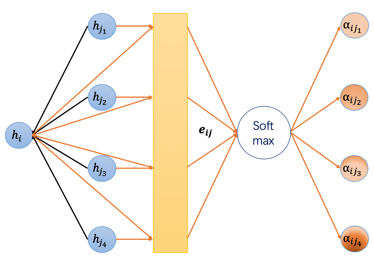
What kind of attention distribution has our model learnt?
Because the attention weight is associated with edges, we can
visualize it by coloring edges. Below we pick a subgraph of Cora and plot the
attention weights of the last GATLayer. The nodes are colored according to
their labels, whereas the edges are colored according to the magnitude of the
attention weights, which can be referred with the colorbar on the right.
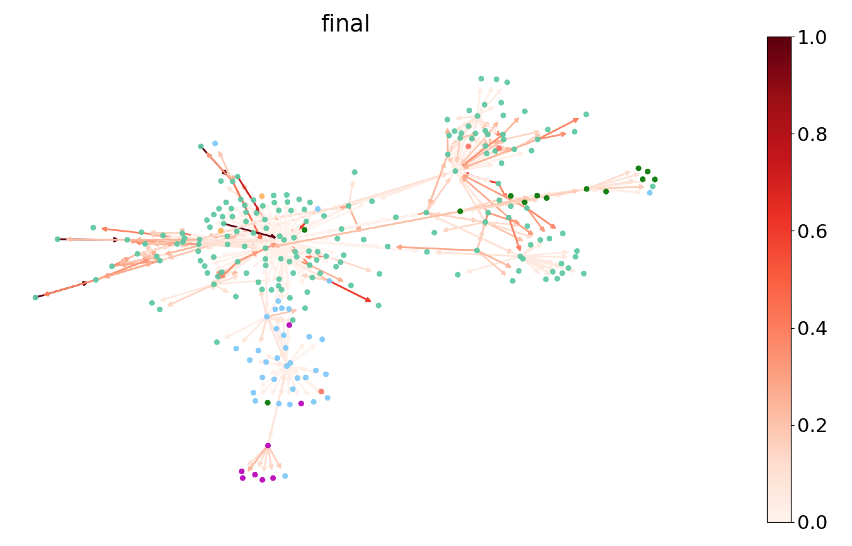
You can that the model seems to learn different attention weights. To understand the distribution more thoroughly, we measure the entropy of the attention distribution. For any node , forms a discrete probability distribution over all its neighbors with the entropy given by
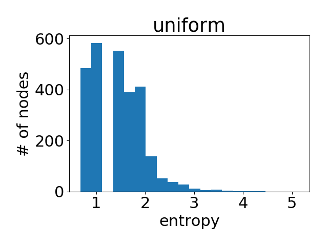
Intuitively, a low entropy means a high degree of concentration, and vice versa; an entropy of 0 means all attention is on one source node. The uniform distribution has the highest entropy of . Ideally, we want to see the model learns a distribution of lower entropy (i.e, one or two neighbors are much more important than the others).
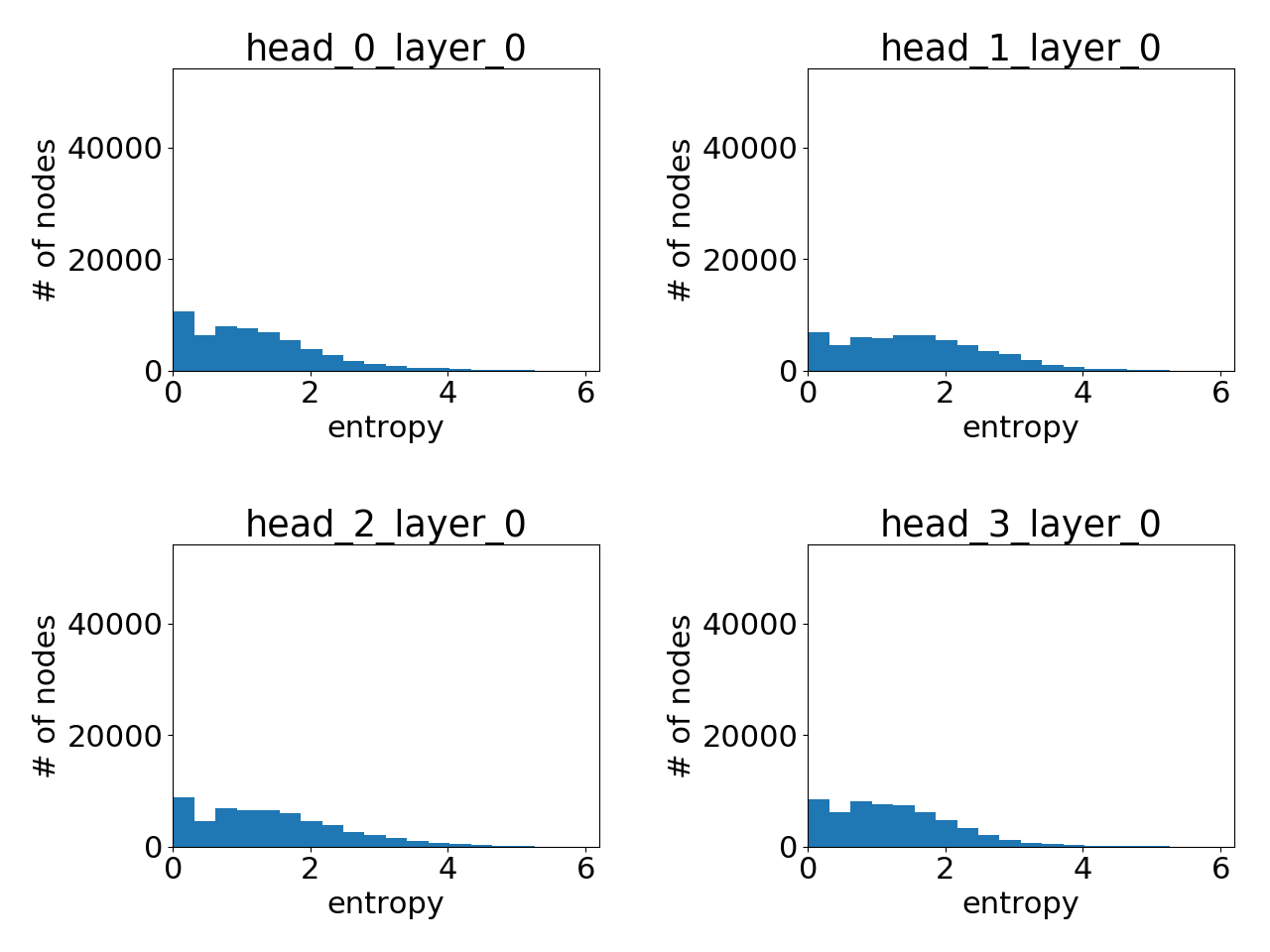
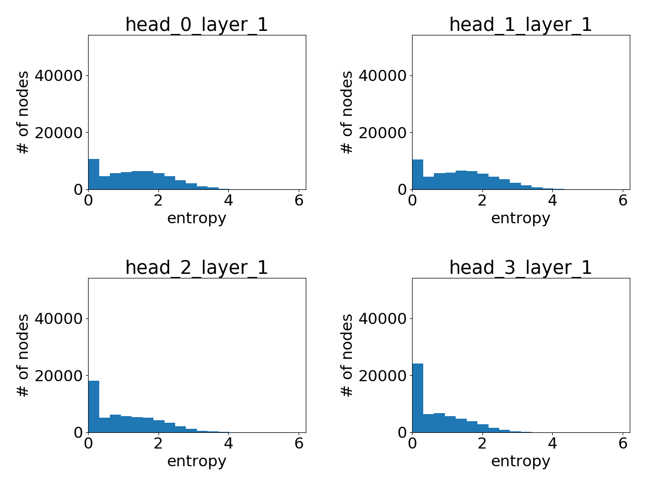
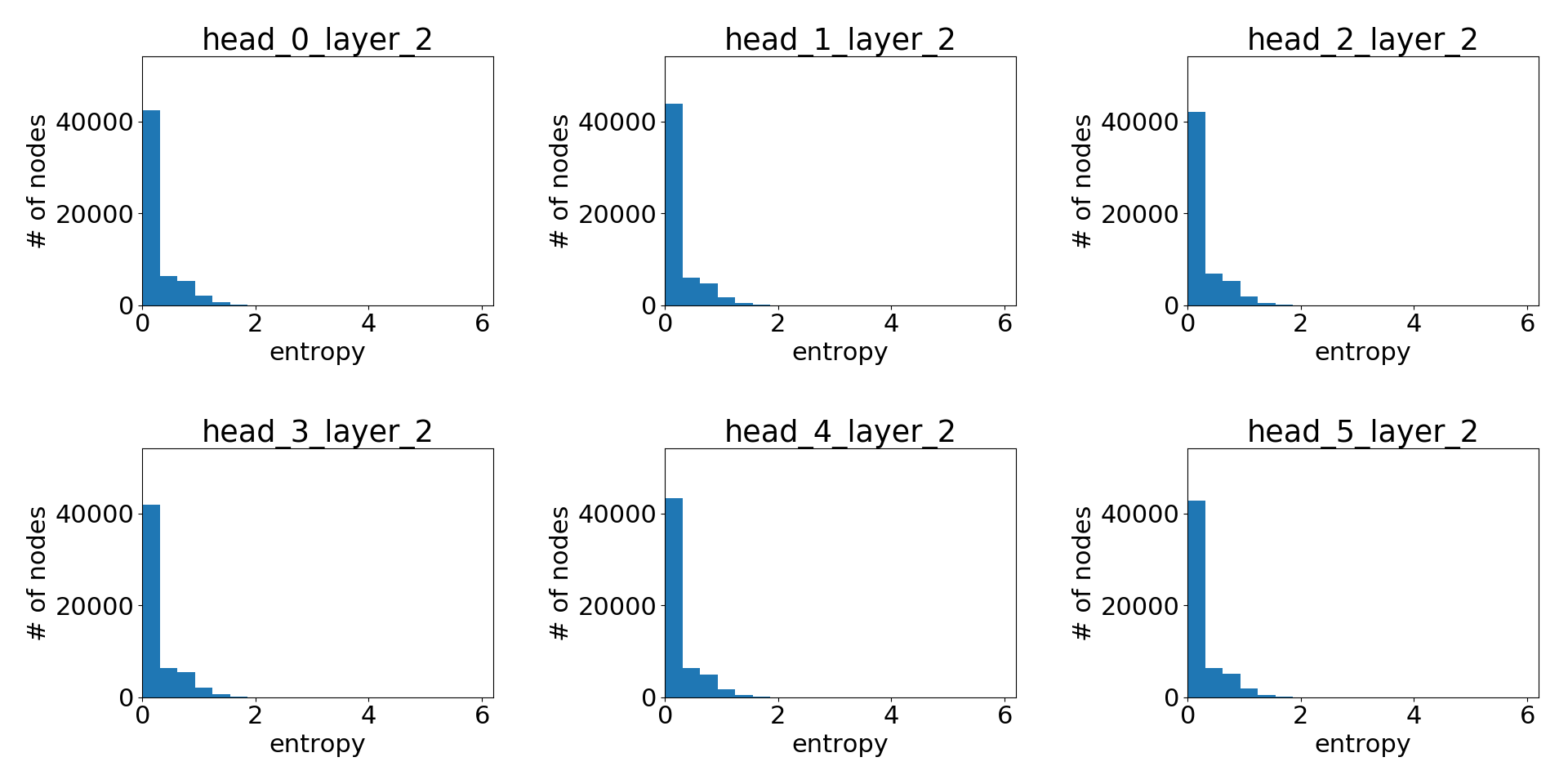
Note that since nodes can have different degrees, the maximum entropy will also be different. Therefore, we plot the aggregated histogram of entropy values of all nodes in the entire graph. Below are the attention histogram of learned by each attention head.
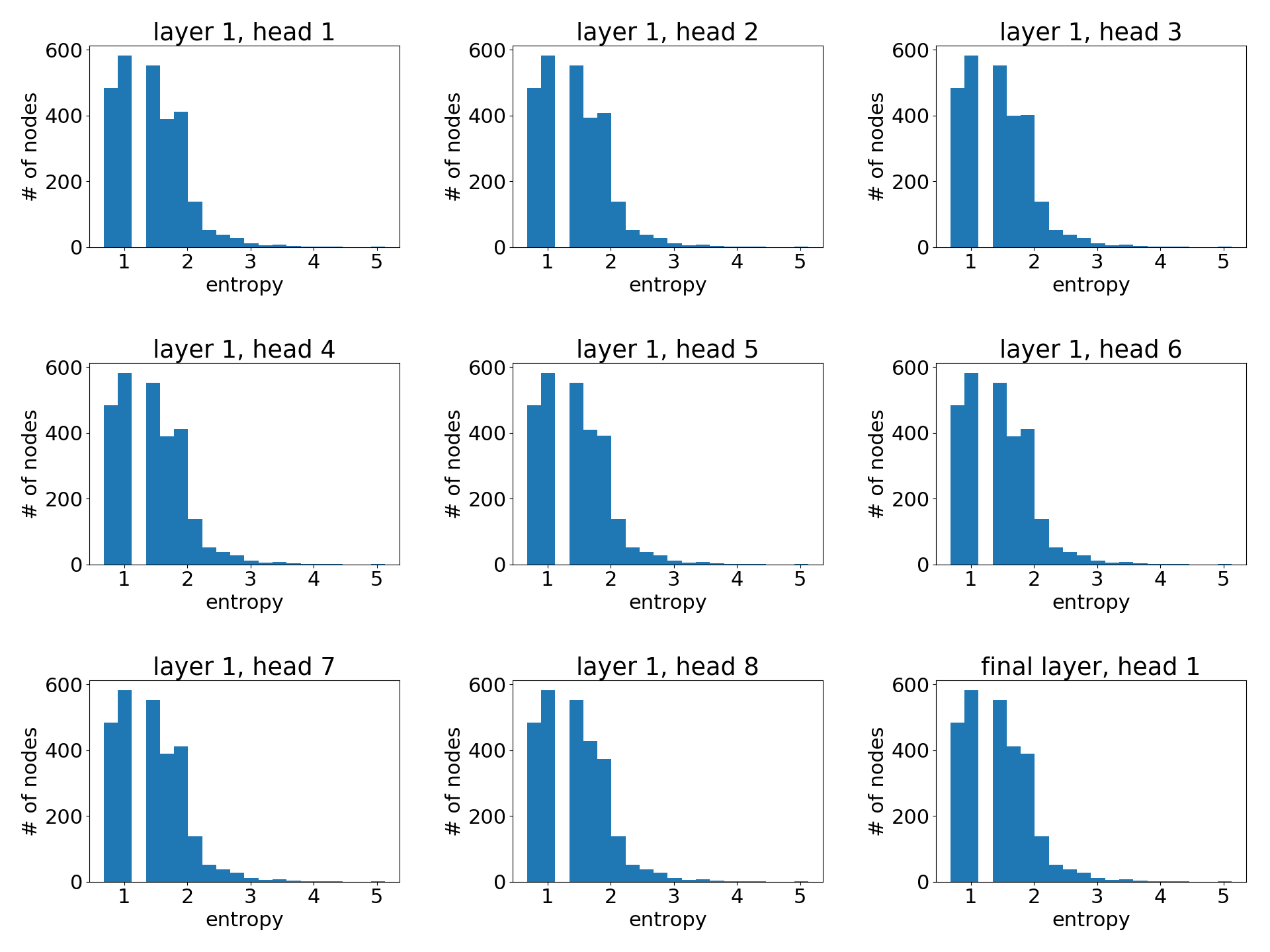
As a reference, here is the histogram if all the nodes have uniform attention weight distribution.
One can see that the attention values learned is quite similar to uniform distribution (i.e, all neighbors are equally important). This partially explains why the performance of GAT is close to that of GCN on Cora (according to author’s reported result, the accuracy difference averaged over runs is less than %); attention does not matter since it does not differentiate much any ways.
Does that mean the attention mechanism is not useful? No! A different dataset exhibits an entirely different pattern, as we show next.
Protein-Protein Interaction (PPI) networks
The PPI dataset used here consists of graphs corresponding to different human tissues. Nodes can have up to kinds of labels, so the label of node is represented as a binary tensor of size . The task is to predict node label.
We use graphs for training, for validation and for test. The average number of nodes per graph is . Each node has features that are composed of positional gene sets, motif gene sets and immunological signatures. Critically, test graphs remain completely unobserved during training, a setting called “inductive learning”.
We compare the performance of GAT and GCN for random runs on this task and use hyperparameter search on the validation set to find the best model.
| Model | F1 Score(micro) |
|---|---|
| GAT | |
| GCN | |
| Paper |
The table above is the result of this experiment, where we use micro F1 score to evaluate the model performance.
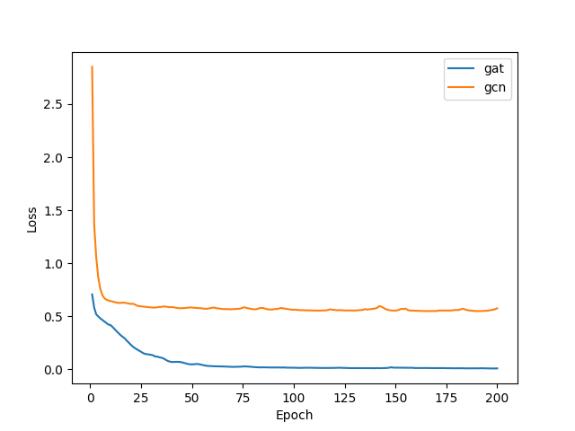
During training, we use BCEWithLogitsLoss as the loss function. The learning
curves of GAT and GCN are presented below; what is evident is the dramatic
performance adavantage of GAT over GCN.
As before, we can have a statistical understanding of the attentions learnt by showing the histogram plot for the node-wise attention entropy. Below are the attention histogram learnt by different attention layers.
Attention learnt in layer 1:
Attention learnt in layer 2:
Attention learnt in final layer:
Again, comparing with uniform distribution:
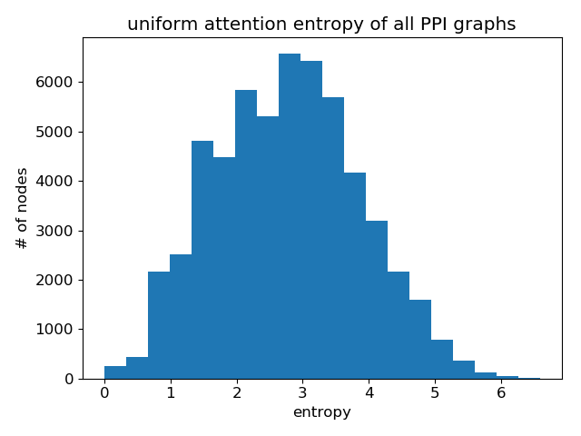
Clearly, GAT does learn sharp attention weights! There is a clear pattern over the layers as well: the attention gets more sharper with higher layer.
Unlike the Cora dataset where GAT’s gain is lukewarm at best, for PPI there is a significant performance gap between GAT and other GNN variants compared in the GAT paper (at least %), and the attention distributions between the two clearly differ. While this deserves further research, one immediate conclusion is that GAT’s advantage lies perhaps more in its ability to handle a graph with more complex neighborhood structure.
What’s Next?
So far, we demonstrated how to use DGL to implement GAT. There are some missing details such as dropout, skip connections and hyper-parameter tuning, which are common practices and do not involve DGL-related concepts. We refer interested readers to the full example.
- See the optimized full example here.
- Stay tune for our next tutorial about how to speedup GAT models by parallelizing multiple attention heads and SPMV optimization.
17 February
By Hao Zhang, Mufei Li, Minjie Wang, Zheng Zhang, in blog