Batched Graph Classification with DGL

Graph classification is an important problem with applications across many fields – bioinformatics, chemoinformatics, social network analysis, urban computing and cyber-security. Applying graph neural networks to this problem has been a popular approach recently (Ying et al., 2018, Cangea et al., 2018, Knyazev et al., 2018, Bianchi et al., 2019, Liao et al., 2019, Gao et al., 2019).

This tutorial is a demonstration for

• batching multiple graphs of variable size and shape with DGL
• training a graph neural network for a simple graph classification task

Simple Graph Classification Task

In this tutorial, we will learn how to perform batched graph classification with DGL via a toy example of classifying 8 types of regular graphs as below:

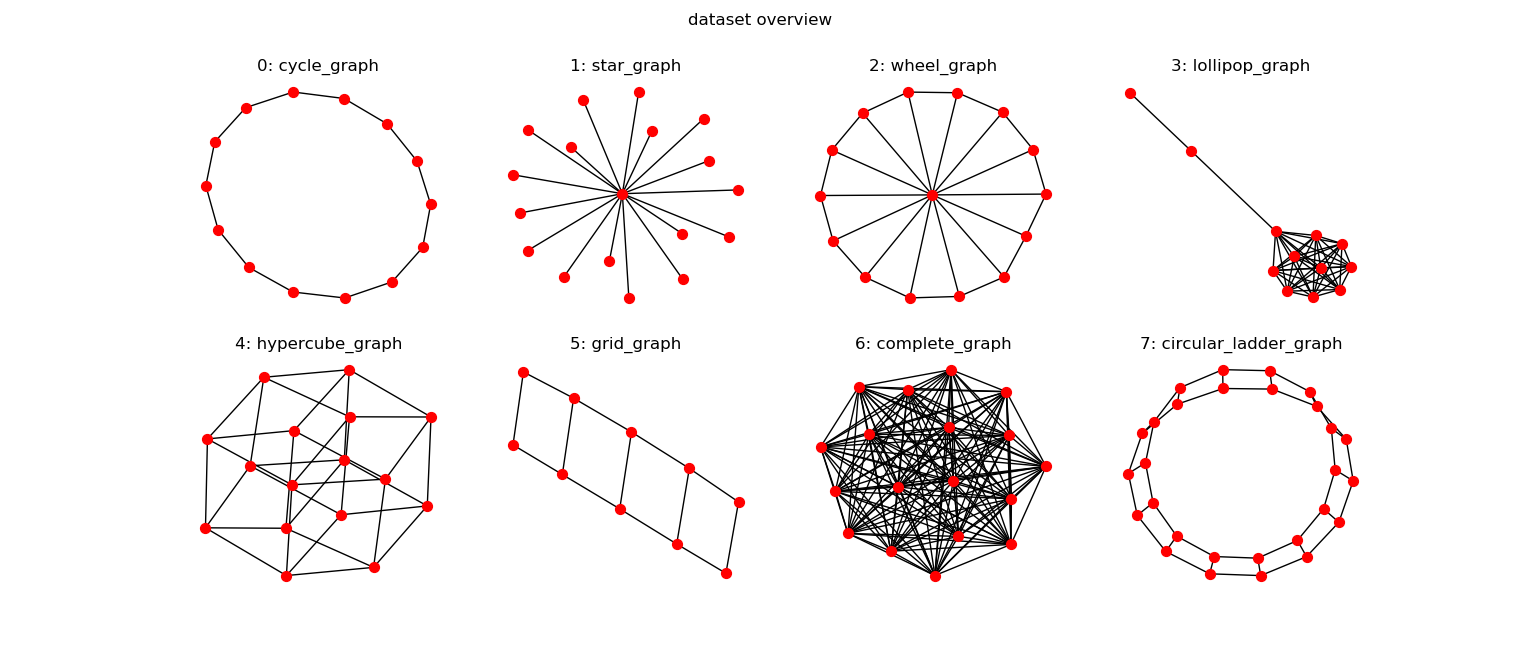
We implement this Mini Graph Classification Dataset in DGL. The dataset has 8 different types of graphs and each class has the same number of graph samples.

from dgl.data import MiniGCDataset
import networkx as nx
# a dataset with 80 samples, each graph is
#  of size [10, 20]
dataset = MiniGCDataset(80, 10, 20)
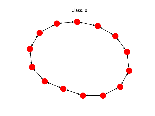
graph, label = dataset[0]
nx.draw(graph.to_networkx())
print('Class:', label)

Form a graph mini-batch

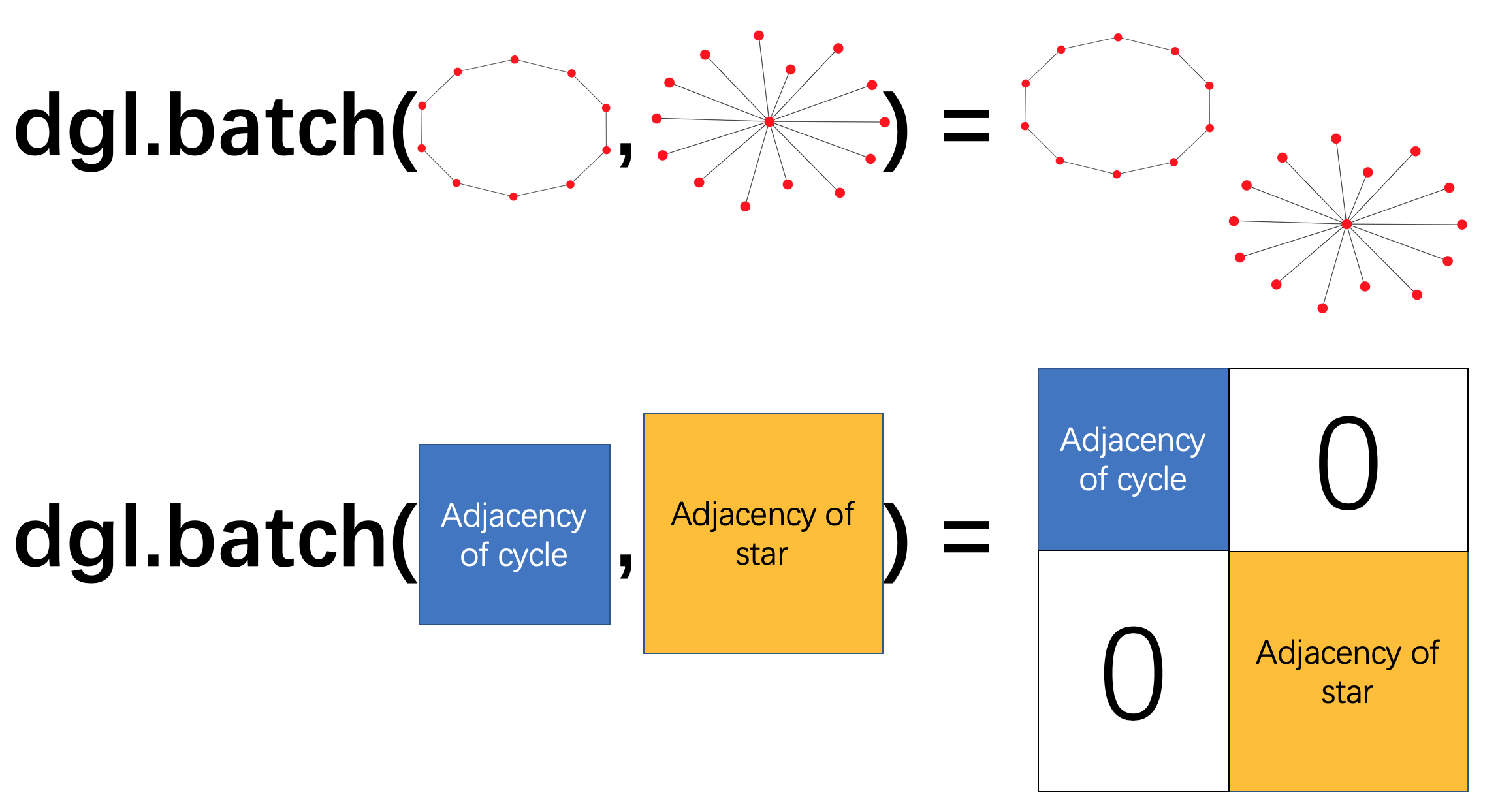
To train neural networks more efficiently, a common practice is to batch multiple samples together to form a mini-batch. Batching fixed-shaped tensor inputs is quite easy (for example, batching two images of size 28x28 gives a tensor of shape 2x28x28). By contrast, batching graph inputs has two challenges:

• Graphs are sparse.
• Graphs can have various length (e.g. number of nodes and eges).

To address this, DGL provides a dgl.batch API. It leverages the trick that a batch of graphs can be viewed as a large graph that have many disjoint connected components. Below is a visualization that gives the general idea:

For example, we can define the following collate function to form a mini-batch from a given list of graph and label pairs (as provided by the MiniGCDataset):

def collate(samples):
    # The input `samples` is a list of pairs
    #  (graph, label).
    graphs, labels = map(list, zip(*samples))
    batched_graph = dgl.batch(graphs)
    return batched_graph, torch.tensor(labels)

The return type of dgl.batch is still a graph (similar to the fact that a batch of tensors is still a tensor). This means that any code that works for one graph immediately works for a batch of graphs. More importantly, since DGL processes messages on all nodes and edges in parallel, this greatly improves efficiency.

Graph Classifier

The graph classification can be proceeded as follows:

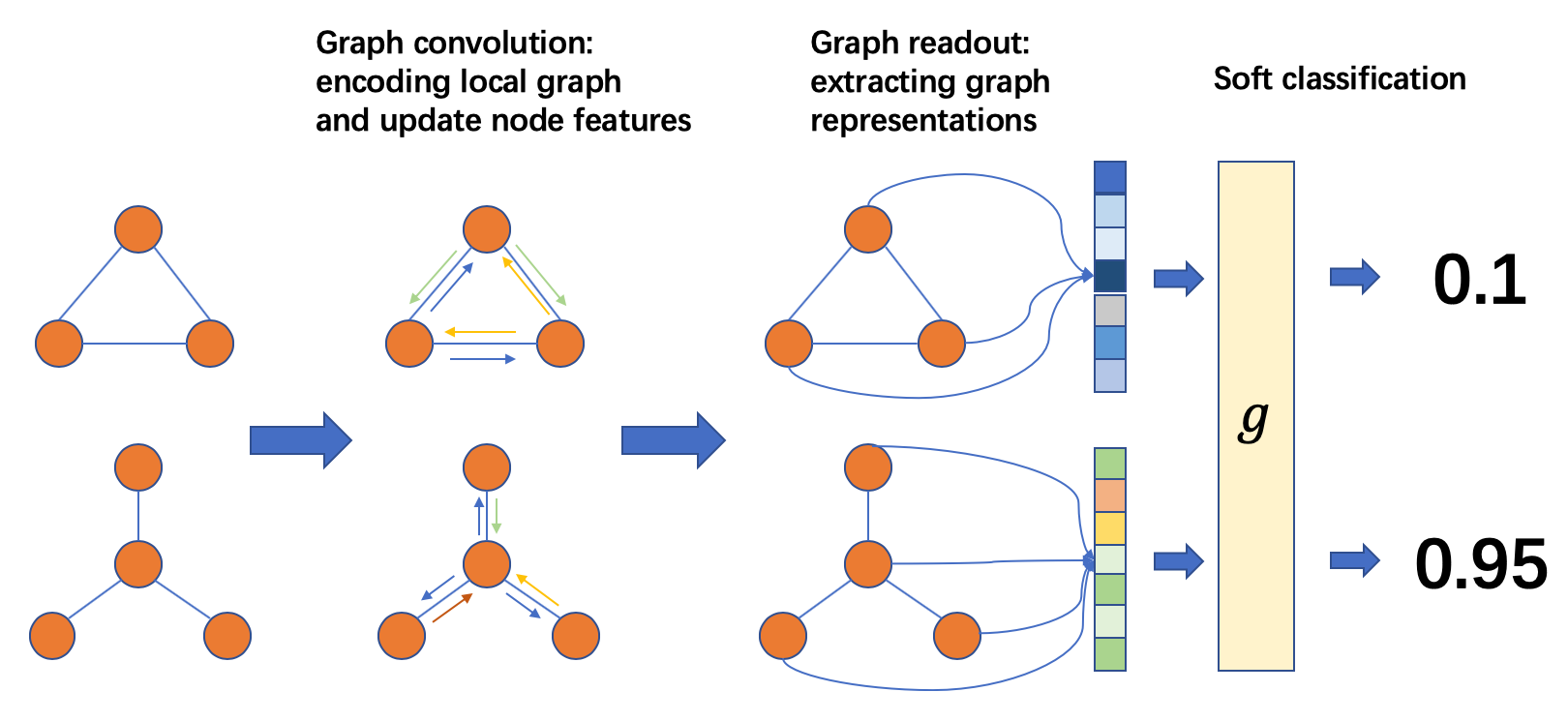
From a batch of graphs, we first perform message passing/graph convolution for nodes to “communicate” with others. After message passing, we compute a tensor for graph representation from node (and edge) attributes. This step may be called “readout/aggregation” interchangeably. Finally, the graph representations are fed into a classifier to predict the graph labels.

Graph Convolution

Our graph convolution operation is basically the same as that for GCN (checkout our earlier tutorial on GCN). The only difference is that we replace $h_{v}^{(l+1)} = \text{ReLU}\left(b^{(l)}+\sum_{u\in\mathcal{N}(v)}h_{u}^{(l)}W^{(l)}\right)$ by $h_{v}^{(l+1)} = \text{ReLU}\left(b^{(l)}+\frac{1}{|\mathcal{N}(v)|}\sum_{u\in\mathcal{N}(v)}h_{u}^{(l)}W^{(l)}\right)$. The replacement of summation by average is to balance nodes with different degrees, which gives a better performance for this experiment.

Note that the self edges added in the dataset initialization allows us to include the original node feature $h_{v}^{(l)}$ when taking the average. Below is the code snipplet to implement this GCN in DGL.

import dgl.function as fn
import torch
import torch.nn as nn

# Sends a message of node feature h.
msg = fn.copy_src(src='h', out='m')

def reduce(nodes):
    """Take an average over all neighbor node features hu and use it to
    overwrite the original node feature."""
    accum = torch.mean(nodes.mailbox['m'], 1)
    return {'h': accum}

class NodeApplyModule(nn.Module):
    """Update the node feature hv with ReLU(Whv+b)."""
    def __init__(self, in_feats, out_feats, activation):
        super(NodeApplyModule, self).__init__()
        self.linear = nn.Linear(in_feats, out_feats)
        self.activation = activation

    def forward(self, node):
        h = self.linear(node.data['h'])
        h = self.activation(h)
        return {'h' : h}

class GCN(nn.Module):
    def __init__(self, in_feats, out_feats, activation):
        super(GCN, self).__init__()
        self.apply_mod = NodeApplyModule(in_feats, out_feats, activation)

    def forward(self, g, feature):
        # Initialize the node features with h. 
        g.ndata['h'] = feature
        g.update_all(msg, reduce)
        g.apply_nodes(func=self.apply_mod)
        return g.ndata.pop('h')

Readout and Classification

For this demonstration, we consider initial node features to be their degrees. After two rounds of graph convolution, we perform a graph readout by averaging over all node features for each graph in the batch:

In DGL, dgl.mean_nodes(g) handles this task for a batch of graphs with variable size. We then feed our graph representations into a classifier with one linear layer followed by $\text{sigmoid}$.

import torch.nn.functional as F

class Classifier(nn.Module):
    def __init__(self, in_dim, hidden_dim, n_classes):
        super(Classifier, self).__init__()
        self.layer0 = GCN(in_dim, hidden_dim, F.relu)
        self.layer1 = GCN(hidden_dim, hidden_dim, F.relu)
        self.classify = nn.Linear(hidden_dim, n_classes)

    def forward(self, g):
        # For undirected graphs, in_degree is the same as
        # out_degree.
        h = g.in_degrees().view(-1, 1).float()
        h = layer0(g, h)
        h = layer1(g, h)
        g.ndata['h'] = h
        hg = dgl.mean_nodes(g, 'h')
        return self.classify(hg)

Setup and Training

We create a synthetic dataset of 1000 graphs with 10 - 20 nodes.

from torch.utils.data import DataLoader
import torch.optim as optim
from dgl.data import MiniGCDataset

# Create training and testing set.
trainset = MiniGCDataset(1000, 10, 20)
testset = MiniGCDataset(200, 10, 20)
# Use pytorch's DataLoader and the collate function
# defined before.
data_loader = DataLoader(trainset, batch_size=32, shuffle=True,
                         collate_fn=collate)
# Create model
model = Classifier(1, 32, 8)
loss_func = nn.CrossEntropyLoss()
optimizer = optim.Adam(model.parameters(), lr=0.001)
model.train()

epoch_losses = []
for epoch in range(50):
    epoch_loss = 0
    for iter, (bg, label) in enumerate(data_loader):
        prediction = model(bg)
        loss = loss_func(prediction, label)
        optimizer.zero_grad()
        loss.backward()
        optimizer.step()
        epoch_loss += loss.detach().item()
    print('Epoch {}, loss {:.4f}'.format(epoch, loss))
    epoch_losses.append(epoch_loss / (iter + 1))

The learning curve of a run is presented below:

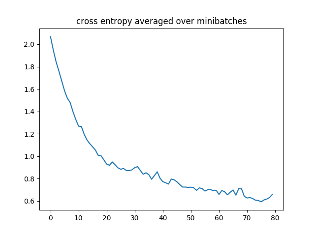
On our test set with the trained classifier, the accuracy of sampled predictions varies across random runs between 78% ~ 85%. The argmax accuracy is typically higher and can reach up to 91%.

# Convert a list of tuples to two lists
model.eval()
test_X, test_Y = map(list, zip(*testset))
test_bg = dgl.batch(test_X)
test_Y = torch.tensor(test_Y).float().view(-1, 1)
probs_Y = torch.softmax(model(test_bg), 1)
sampled_Y = torch.multinomial(probs_Y, 1)
argmax_Y = torch.max(probs_Y, 1)[1].view(-1, 1)
print('Accuracy of sampled predictions on the test set: {:.4f}%'.format(
    (test_Y == sampled_Y.float()).sum().item() / len(test_Y) * 100))
print('Accuracy of argmax predictions on the test set: {:4f}%'.format(
    (test_Y == argmax_Y.float()).sum().item() / len(test_Y) * 100))

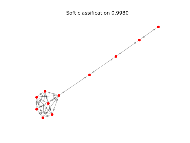
Below is an animation where we plot graphs with the probability a trained model assigns its ground truth label to it:

To understand how the node/graph features change over layers with a trained model, we use t-SNE for dimensionality reduction and visualization.

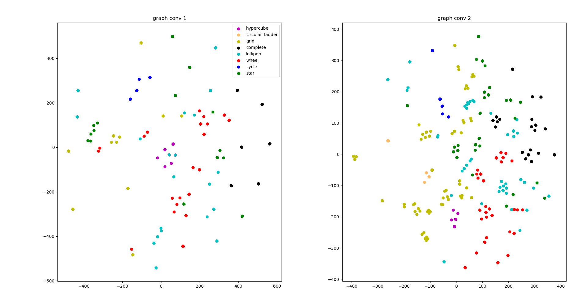
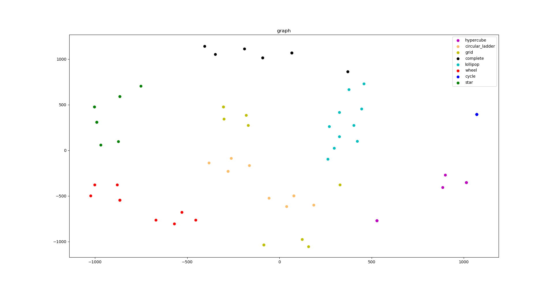
The two small figures on the top separately visualize node features after , graph convolution layer #1 and #2, and the figure on the bottom visualizes the pre-softmax logits for graphs. As you can see, the node embeddings of different types of graphs are more separable in the higher layer and the lower layer. Finally, the embeddings of different types of graphs are well-separated.

What’s Next?

Download the full tutorial code and jupyter notebook here.

Graph classification with graph neural networks is still a very young field waiting for folks to bring more exciting discoveries! It is not easy as it requires mapping different graphs to different embeddings while preserving their structural similarity in the embedding space. To learn more about it, “How Powerful Are Graph Neural Networks?” in ICLR 2019 might be a good starting point.

With regards to more examples on batched graph processing, see:

• our tutorials on Tree LSTM and Deep Generative Models of Graphs
• an example implementation of Junction Tree VAE.